Archive for the ‘theory’ Category

h1

Some research papers on hierarchical models

May 15, 2018

Accurate parameter estimation for Bayesian network classifiers using hierarchical Dirichlet processes”, by François Petitjean, Wray Buntine, Geoffrey I. Webb and Nayyar Zaidi, in Machine Learning, 18th May 2018, DOI 10.1007/s10994-018-5718-0.  Available online at Springer Link.  To be presented at ECML-PKDD 2018 in Dublin in September, 2018.

Abstract This paper introduces a novel parameter estimation method for the probability tables of Bayesian network classifiers (BNCs), using hierarchical Dirichlet processes (HDPs).  The main result of this paper is to show that improved parameter estimation allows BNCs  to outperform leading learning methods such as random forest for both 0–1 loss and RMSE,  albeit just on categorical datasets. As data assets become larger, entering the hyped world of “big”, efficient accurate classification requires three main elements: (1) classifiers with low bias that can capture the fine-detail of large datasets (2) out-of-core learners that can learn from data without having to hold it all in main memory and (3) models that can classify new data very efficiently. The latest BNCs satisfy these requirements. Their bias can be controlled easily by increasing the number of parents of the nodes in the graph. Their structure can be learned out of core with a limited number of passes over the data. However, as the bias is made lower to accurately model classification tasks, so is the accuracy of their parameters’ estimates, as each parameter is estimated from ever decreasing quantities of data. In this paper, we introduce the use of HDPs for accurate BNC parameter estimation even with lower bias. We conduct an extensive set of experiments on 68 standard datasets and demonstrate that our resulting classifiers perform very competitively with random forest in terms of prediction, while keeping the out-of-core capability and superior classification time.
Keywords Bayesian network · Parameter estimation · Graphical models · Dirichlet 19 processes · Smoothing · Classification

“Leveraging external information in topic modelling”, by He Zhao, Lan Du, Wray Buntine & Gang Liu, in Knowledge and Information Systems, 12th May 2018, DOI 10.1007/s10115-018-1213-y.  Available online at Springer Link.  This is an update of our ICDM 2017 paper.

Abstract Besides the text content, documents usually come with rich sets of meta-information, such as categories of documents and semantic/syntactic features of words, like those encoded in word embeddings. Incorporating such meta-information directly into the generative process of topic models can improve modelling accuracy and topic quality, especially in the case where the word-occurrence information in the training data is insufficient. In this article, we present a topic model called MetaLDA, which is able to leverage either document or word meta-information, or both of them jointly, in the generative process. With two data augmentation techniques, we can derive an efficient Gibbs sampling algorithm, which benefits from the fully local conjugacy of the model. Moreover, the algorithm is favoured by the sparsity of the meta-information. Extensive experiments on several real-world datasets demonstrate that our model achieves superior performance in terms of both perplexity and topic quality, particularly in handling sparse texts. In addition, our model runs significantly faster than other models using meta-information.
Keywords Latent Dirichlet allocation · Side information · Data augmentation ·
Gibbs sampling

“Experiments with Learning Graphical Models on Text”, by Joan Capdevila, He Zhao, François Petitjean and Wray Buntine, in Behaviormetrika, 8th May 2018, DOI 10.1007/s41237-018-0050-3.  Available online at Springer Link.  This is work done by Joan Capdevila during his visit to Monash in 2017.

Abstract A rich variety of models are now in use for unsupervised modelling of text documents, and, in particular, a rich variety of graphical models exist, with and without latent variables. To date, there is inadequate understanding about the comparative performance of these, partly because they are subtly different, and they have been proposed and evaluated in different contexts. This paper reports on our experiments with a representative set of state of the art models: chordal graphs, matrix factorisation, and hierarchical latent tree models. For the chordal graphs, we use different scoring functions. For matrix factorisation models, we use different hierarchical priors, asymmetric priors on components. We use Boolean matrix factorisation rather than topic models, so we can do comparable evaluations. The experiments perform a number of evaluations: probability for each document, omni-directional prediction which predicts different variables, and anomaly detection. We find that matrix factorisation performed well at anomaly detection but poorly on the prediction task. Chordal graph learning performed the best generally, and probably due to its lower bias, often out-performed hierarchical latent trees.
Keywords Graphical models · Document analysis · Unsupervised learning ·
Matrix factorisation · Latent variables · Evaluation


h1

Whither the Scientific Method

January 28, 2018

Long before the Industrial Age in Europe we had the Dark Ages. Popular culture tells us it was believed that the Earth was flat, witches caused the plague, and the ways of the world were decreed by kings, or God himself. While rationalist explanations of the world appeared independently in many ancient civilisations, the scientific method as we know it became prominent in the 19th century as a remarkable series of scientific and engineering discoveries propelled the world into the industrial age.  Indeed, Karl Pearson stated “the scientific method is the sole gateway to the whole region of knowledge.”.

With the pre-eminence of science in our modern society, controversies about science often occur in the media and public discussion, and the list of such areas is large. It doesn’t help that aspects of society, politics or religion have been falsely dressed up with “science,” so-called Scientism.  The expression “the science is settled” is a phrase from global warming skeptics that seeks to align global warning views with scientism (i.e., science is never settled so how can global warming be settled).  Note we can also view the statement “the science is settled” as a Socratian noble lie, therefore justifying its use in public discussion.

So apart from false applications of science, i.e., scientism, what flaws with the scientific method are there?

Flaws in the Science?

Medical science has suffered bad press in recent times. Best known through the popular work of John Ioannidis, provocatively titled “Why Most Published Research Findings Are False”, testaments from famous and authoritative medical researchers about the flaws of published medical research abound. As an empirical computer scientist, I can assure you flaws in research are not restricted to medical science, its just that medical science is perhaps our most societally important area of science.

Some of the discussed flaws in research are the misuse of p-values though a variety of means. For an entertaining example, see John Bohannon’s “I Fooled Millions Into Thinking Chocolate Helps Weight Loss.” Other flaws are so-called surrogate endpoints (a biomarker such as a blood test is used as a substitute for a clinical endpoint such as a heart attack), and others still are poorly matched motivations, i.e., for academics, the idea of “publish or perish” but for industry this would be “publish and profit”.  Many lists of flaws have been published.

In all, however, the scientific method holds up as a valid approach because the flaws invariable amount to corruption of the original method. One way the medical community addresses this is by adding an additional layer on top of the standard scientific method, often called the systematic review.  This is where unbiased experts review a series of scientific studies on a particular question, make judgments about the quality of the scientific method and the evidence, and develop recommendations for healthcare. The systematic review is, if you like, quality control for the scientific method.

The End of Theory?

Another seeming assault on the scientific method comes from data science. In 2008 Chris Anderson of Wired published a controversial blog about “The End of Theory”. The idea is that the deluge of data completely changes how we should progress with scientific discovery. We don’t need theory, he claims, we just extract information from the deluge of data. The responses, and there are many, came quickly, for instance Massimo Pigliucci said “But, if we stop looking for models and hypotheses, are we still really doing science?”, and others questions the veracity and appropriateness of much observational data, and hence its suitability as a subject of analysis.

Anderson’s “end of theory,” like John Horgan’s “end of science”, is not so much wrong as much more complex that it first seems. The relationship between data science and the scientific method is not simple. To understand this, consider that the poster child for 19th century science was physics.  Physics, a mathematical science, is fundamentally different to say modern medicine. In physics, Eugene Wigner’s notion of the “unreasonable effectiveness of mathematics” holds sway: from a concise theory we can derive enormous consequences. A relatively small amount of well chosen scientific hypotheses have uncovered vast regions of the engineering and physics universe. For instance, weather predictions are currently based on simulations built using the Newtonian laws of physics coupled with geophysical and weather data.

The imbalance (a small number of scientific hypotheses needed to justify a large area of science) indeed suits the scientific method. Peter Norvig, however, points out this is not feasible in areas such as biology and medical science, where the unreasonable effectiveness of mathematics does not hold. In these areas, the complexities of the underlying processes means we cannot necessarily simulate the impact of a eating raw cocoa or drinking red wine on heart health because the simulation or derivations from fundamental properties of nature are just too complex.

Norvig’s colleagues at Google, some of the founders of data science, instead refer to the unreasonable effectiveness of data. That is, fundamental complexity of some sciences mean we should instead be using data-driven processes for discovery of scientific details.

Data Dredging

To understand how data science can change the scientific method, we need to look at how it should not change it. Statisticians like to talk derisively about data dredging, with p-hacking being the best known example. As in the chocolate study mentioned above, this is where studies are repeated (in some way) until a significant p-value is obtained. They argue data driven discovery is dangerous. But this is the wrong viewpoint for data science. In complex areas like medical science or biology, we have many possible hypotheses and our intuitions can be poor in these complex worlds.

Computer science has an elegant theory of complexity called NP-completeness, which is the notion that one may need to test an exponential number of things before finding one that works.  A closer notion, though, is sample complexity.  This is the number of training cases we need to learn a concept.  In a sequence of experiments to uncover the causal structure of a domain, you are actively choosing the experiments sequentially, so a closer notion is the sample complexity of active learning.  While some theory exists here, and the numbers are no longer exponential, the results are not great.  A scientist could expect to be running an awful lot of experiments!  So this is the situation we find ourselves with hypothesis testing in the broader scientific world where the unreasonable effectiveness of mathematics fails.

In the early days of machine learning I worked at Prof. Ross Quinlan’s lab in Sydney. We soon discovered our own version of Ioannidis’ flaws in medical science that applied to machine learning. We called it theory overfitting, in contrast to regular overfitting which is an artifact of the bias-variance dilemma in statistics and machine learning. People tested a bunch of different theories on a small number, say 5 data sets, and eventually they find one that works, and so write it up and publish it. In truth its just another variant of p-hacking.

In data science, if we’re appling machine learning or neural network algorithms to a body of data, we are invariably trying to solve an NP-complete problem and are thus subject to overfitting or p-hacking. Even if we employ careful statistical methods to try to overcome this, we may subsequently be doing theory overfitting. However, if we don’t employ machine learning methods, we may never uncover reasonable hypotheses in the large pool of candidates. T his is the conundrum of data science for the scientific method when used in broader non-mathematical domains.

Powering the Scientific Method

Organisations and hard nose businesses have this conundrum effectively solved. At Kaggle for instance, and in TREC competitions, a test data set is always hidden from the machine learners, and only used for a final validation, which acts like a (final) cycle of the scientific method. The initial “develop a general theory” step of the scientific method has been done with machine learning. This can be considered to be millions of embedded hypothesise-test cycles. Thus we have an epicycle view of the scientific method.

But applying this approach in the medical world is not straight forward.  The medical research world keeps data registries that feasibly can be used to obtain data for discovery purposes. However, to obtain data, one usually has to apply for ethics clearance/approval, that the intended use of the data is good. The ethics committees who oversee the approval are the gatekeepers of data, and oftentimes they expect to see a valid scientific plan, not an open-ended discovery proposal. With the epicycle view of the scientific method, registries, when they release data for discovery exercises, would need to withhold some data for a final validation step in order to preserve the validity of the scientific method.

h1

Notes on Determinantal Point Processes

September 11, 2017
Wray at Yandex Sept 2017

Wray at Yandex Sept 2017 with Prof. Konstantin Vorontsov, Anna Potapenko and others in his group.

I’m giving a tutorial on these amazing processes while in Moscow.  The source “book” for this is of course Alex Kulesza and Ben Taskar’s, “Determinantal Point Processes for Machine Learning”, Foundations and Trends® in Machine Learning: Vol. 5: No. 2–3, pp 123-286, 2012.  The full lecture I gave at Yandex is here.

If you have an undergraduate in mathematics with loads of multi-linear algebra and real analysis, this stuff really is music for the mind.  The connections and results are very cool.  In my view these guys don’t spend enough time in their intro. on gram matrices, which really is the starting point for everything.  In their online video tutorials they got this right, and lead with these results.

There is also a few interesting connections they didn’t mention.  Anyway, I did some additional lecture notes to give some of the key results mentioned in the long article and elsewhere that didn’t make their tutorial slides.

h1

Advanced Methodologies for Bayesian Networks

August 22, 2017

The 3rd Workshop on Advanced Methodologies for Bayesian Networks was run in Kyoto September 20-22, 2017. The workshop was well organised, and the talks were great. Really good invited talks by great speakers!

I’ll be talking about our (with François Petitjean, Nayyar Zaidi and Geoff Webb) recent work with Bayesian Network Classifiers:

Backoff methods for estimating parameters of a Bayesian network

Various authors have highlighted inadequacies of BDeu type scores and this problem is shared in parameter estimation. Basically, Laplace estimates work poorly, at least because setting the prior concentration is challenging. In 1997, Freidman et al suggested a simple backoff approach for Bayesian network classifiers (BNCs). Backoff methods dominate in in n-gram language models, with modified Kneser-Ney smoothing, being the best known, and a Bayesian variant exists in the form of Pitman-Yor process language models from Teh in 2006. In this talk we will present some results on using backoff methods for Bayes network classifiers and Bayesian networks generally. For BNCs at least, the improvements are dramatic and alleviate some of the issues of choosing too dense a network.

Slides are at the AMBN site, here.  Note I spent a bit of time embellishing my slides with some fabulous historical Japanese artwork!

Software for the system is built on the amazing Chordalysis system of François Petitjean, and the code is available as HierarchicalDirichletProcessEstimation.  Boy, Nayyar and François really can do good empirical work!

h1

Lectures: Bayesian Learning with Graphical Models

July 15, 2017

I’m giving a series of lectures this semester combining graphical models and some elements of nonparametric statistics within the Bayesian context.  The intent is to build up to the theory of discrete matrix factorisation and its many variations. The lectures start on 27th July and are mostly given weekly.  Weekly details are given in the calendar too.  The slides are on the Monash share drive under “Wray’s Slides” so if you are at Monash, do a search on Google drive to find them.  If you cannot find them, email me for access.

OK lectures over as of 24/10/2017!  Have some other things to prepare.

Variational Algorithms and Expectation-Maximisation, Lecture 6, 19/10/17, Wray Buntine

This week takes up on material not covered last lecture.  For exponential family distributions, working with the mean of Gibbs samples sometimes sometimes corresponds to another algorithm called Expectation-Maximisation. We will look at this in terms of the Kullback-Leibler versions of variational algorithms. The general theory is quite involved, so we will work through it with some examples, like variational auto-encoders, Gaussian mixture models, and extensions to LDA.

No lectures this week, 12th October, as I will be catching up on reviews and completing a journal article. Next week we’ll work through some examples of variational algorithms, including LDA with a HDP, a model whose VA theory has been thoroughly botched up historically.

Gibbs Sampling, Variational Algorithms and Expectation-Maximisation, Lecture 5, 05/10/17, Wray Buntine

Gibbs sampling is the simplest of the Monte Carlo Markov Chain methods, and the easiest to understand. For computer scientists, it is closely related to local search. We will look at the basic justification of Gibbs sampling and see examples of its variations: block Gibbs, augmentation and collapsing. Clever use of these techniques can dramatically improve performance. This gives a rich class of algorithms that, for smaller data sets at least, addresses most problems in learning. For exponential family distributions, taking the mean instead of sampling sometimes corresponds to another algorithm called Expectation-Maximisation. We will look at this in terms of the Kullback-Leibler versions of variational algorithms. We will look at the general theory and some examples, like variational auto-encoders and Gaussian mixture models.

ASIDE: Determinantal Point Processes, one off lecture, 28/09/17, Wray Buntine

Representing objects with feature vectors lets us measure similarity using dot products.  Using this notion, the determinantal point process (DPP) can be introduced as a distribution over objects maximising diversity.  In this tutorial we will explore the DPP with the help of the visual analogies developed by Kulesza and Taskar in their tutorials and their 120 page Foundations and Trends article “Determinantal Point Processes for Machine Learning.” Topics covered are interpretations and definitions, probability operations such as marginalising and conditioning, and sampling.  The tutorial makes great use of the knowledge of matrices and determinants.

No lectures the following two weeks, 14th and 21st September, as I will be on travel.

Basic Distributions and Poisson Processes, Lecture 4, 07/09/17, Wray Buntine

We review the standard discrete distributions, relationships, properties and conjugate distributions.  This includes deriving the Poisson distribution as an infinitely divisible distribution on natural numbers with a fixed rate.  Then we introduce Poisson point processes as a model of stochastic processes.  We show how they behave in both the discrete and continuous case, and how they have both constructive and axiomatic definitions.  The same definitions can be extended to any infinitely divisible distributions, so we use this to introduce the gamma process.  We illustrate Bayesian operations for the gamma process: data likelihoods, conditioning on discrete evidence and marginalising.

Directed and Undirected Independence Models, Lecture 3, 31/08/17, Wray Buntine

We will develop the basic properties and results for directed and undirected graphical models.  This includes testing for independence, developing the corresponding functional form, and understanding probability operations such as marginalising and conditioning.  To complete this section, we will also investigate operations on clique trees, to illustrate the principles.  We will not do full graphical model inference.

Information and working with Independence, Lecture 2, 17/08/17, Wray Buntine

This will continue with information (entropy) left over from the previous lecture.  Then we will look at the definition of independence and the some independence models, including its relationship with causality.  Basic directed and undirected models will be introduced.  Some example problems will be presented (simply) to tie these together:  simple bucket search, bandits, graph colouring and causal reasoning.

No lectures 03/08 (writing for ACML) and 10/08 (attending ICML).

Motivating Probability and Decision Models, Lecture 1, 27/07/17, Wray Buntine

This is an introduction to motivation for using Bayesian methods, these days called “full probability modelling” by the cognoscenti, to avoid prior cultish associations and implications. We will look at modelling, causality, probability as frequency, and axiomatic underpinnings for reasoning, decisions, and belief . The importance of priors and computation form the basis of this.


h1

On the “world’s best tweet clusterer” and the hierarchical Pitman–Yor process

July 30, 2016

Kar Wai Lim has just been told they “confirmed the approval” of his PhD (though it hasn’t been “conferred” yet, so he’s not officially a Dr., yet) and he spent the time post submission pumping out journal and conference papers.  Ahhh, the unencumbered life of the fresh PhD!

This one:

“Nonparametric Bayesian topic modelling with the hierarchical Pitman–Yor processes”, Kar Wai Lim , Wray Buntine, Changyou Chen, Lan Du, International Journal of Approximate Reasoning78 (2016) 172–191.

includes what I believe is the world’s best tweet clusterer.  Certainly blows away the state of the art tweet pooling methods.  Main issue is that the current implementation only scales to a million or so tweets, and not the 100 million or expected in some communities.  Easily addressed with a bit of coding work.

We did this to demonstrate the rich possibilities in terms of semantic hierarchies one has, largely unexplored, using simple Gibbs sampling with Pitman-Yor processes.   Lan Du (Monash) started this branch of research.  I challenge anyone to do this particular model with variational algorithms 😉   The machine learning community in the last decade unfortunately got lost on the complexities of Chinese restaurant processes and stick-breaking representations for which complex semantic hierarchies are, well, a bit of a headache!

h1

What “50 Years of Data Science” Leaves Out

November 28, 2015

This blog post from Sean Owen, Director, Data Science @Cloudera / London

I was so glad to find David Donoho’s critical take in 50 Years of Data Science, which has made its way around the Internet. … Along the way to arguing that Data Science can’t be much more than Statistics, it fails to contemplate Data Engineering, which I’d argue is most of what Data Science is and Statistics is not.

Much as I enjoyed reading Donoho’s work, I think its important for people to realise that Data Science isn’t just a new take on applied statistics, a superset yes, but an important superset.

Some additional comments:

  • Donoho like Breiman before him splits Statistics/Machine Learning into Generative versus Predictive modelling.  I never really understand this because near 40% of published ML is generative modelling, and the majority of my work.
  • Other important aspects of Data Science we cover in our Monash course are:
    • data governance and data provenance
    • the business processes and “operationalisation” (putting the results to work to achieve value)
    • getting data, fusing different kinds of data, envisaging data science projects
  • These are above and beyond the area of Greater Data Science (Donoho, section 8) that we refer to as the Data Analysis Process, and is probably the most in-demand skill for what the industry calls a data scientist.

Also, as a Machine Learning guy, who’s been doing Computational Statistics for 25 years, I also think its important to point out that Machine Learning exists as a separate field because their are so many amazing and challenging tasks to do in areas like robotics, natural language processing and image processing.  These require statistical ingenuity, domain understanding, and computational trickery.   I have important contacts both in the Statistical community and the NLP community so I can do my work.


h1

Basic tutorial: Oldie but a goody …

November 7, 2015

A student reminded me of Gregor Heinrich‘s excellent introduction to topic modelling, including a great introduction to the underlying foundations like Dirichlet distributions and multinomials.  Great reading for all students!  See

  • G. Heinrich, Parameter estimation for text analysis, Technical report, Fraunhofer IGD, 15 September 2009 at his publication page.
h1

Some diversions

July 4, 2015

Quora‘s answers on What are good ways to insult a Bayesian statistician?   Excellent.  I’m insulted 😉

Great Dice Data: How Tech Skills Connect.  “Machine learning” is there (case sensitive) under the Data Science cluster in light green.

Data scientist payscales: “machine learning”‘ raises your expected salary but “MS SQL server” lowers it!

Cheat sheetsMachine Learning Cheat Sheet and the Probability Cheat Sheet.   Very handy!

h1

Dirichlet-multinomial distribution versus Pitman-Yor-multinomial

March 18, 2015

If you’re familiar with the Dirichlet distribution as the workhorse for discrete Bayesian modelling, then you should know about the Dirichlet-multinomial.  This is what happens when you combine a Dirichlet with a multinomial and integrate/marginalise out the common probability vector.

Graphically, you have a probability vector \vec\theta 
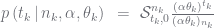
that is the mean for a probability vector \vec{p}.  You then have data, a count vector \vec{n}, drawn using a multinomial distribution with mean \vec{p}. If we integrate out the vector \vec{p} then we get the Dirichlet-multinomial.MDNdata

The standard formulation is to have:
\vec{p} \sim \mbox{Dirichlet}\left(\alpha,\vec\theta\right) ~~~~~~~~~~~~  \vec{n} \sim \mbox{Multinomial}\left(\vec{p},N\right)

Manipulating this, we get the distribution for the Dirichlet-multinomial:
p\left( \vec{n}\,\middle\vert\, \alpha,\vec\theta,N, \mbox{\small Dirichlet-multi.}\right)
~~~~~~~~~~~~=~  \frac{1}{\mbox{\small Beta}(\alpha \vec\theta)}{N \choose \vec{n} }  \int_{\mbox{\scriptsize simplex}} \prod_k p_{k}^{n_k+\alpha \theta_k-1}  \mbox{d}\vec{p}
~~~~~~~~~~~~=~  {N \choose \vec{n} }  \frac{\mbox{\small Beta}(\vec{n}+\alpha \vec\theta)}{\mbox{\small Beta}(\alpha \vec\theta)}

Now we will rewrite this into the Pochhammer symbol notation we use for Pitman-Yor marginals,

(c|d)_{T} is the Pochhammer symbol (a generalised version is used, and a different notation) which is a form of rising factorial so its given by c (c+d) (c+2d) ... (c+(T-1)d); can be computed using Gamma functions
(c)_{T} (special case) a related rising factorial given by c (c+1) (c+2) ... (c+(T-1)) 
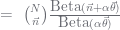
so it corresponds to (c|1)_{T}

The Beta functions simplify to yield the Dirichlet-multinomial in Pochhammer symbol notation:

p\left( \vec{n}\,\middle\vert\, \alpha,\vec\theta,N,\mbox{\small Dirichlet-multi.}\right) ~=~  {N \choose \vec{n} } \frac{1}{(\alpha)_N} \prod_{k=1}^K (\alpha\theta_k)_{n_k}

Now lets do the same with the Pitman-Yor process (PYP).
\vec{p} \sim \mbox{PYP}\left(d,\alpha,\vec\theta\right) ~~~~~~~~~~~~  \vec{n} \sim \mbox{Multinomial}\left(\vec{p},N\right)

The derivation of the combination is more detailed but is found in the Buntine Hutter Arxiv report or my tutorials. For this, you have to introduce a new latent vector \vec{t} where t_k represents the subset of the count n_k that will be passed up from the \vec{p}-node up to the \vec{\theta}-node to convey information about the data \vec{n}.  Keep this phrase in mind.  It will be explained a bit later. These \vec{t} are constrained as follows:

constraint t_k \le n_k
constraint t_k>0 whenever n_k>0
total N=\sum_k n_k
total T=\sum_k t_k

With these, we get the PYP-multinomial in Pochhammer symbol notation:

p\left( \vec{n},\vec{t}\,\middle\vert\, d,\alpha,\vec\theta,N,\mbox{\small PYP-multi.}\right) ~=~ {N \choose \vec{n}}  \frac{(\alpha|d)_T}{(\alpha)_N} \prod_{k = 1}^K \mathcal{S}_{t_k, d}^{n_k} \theta_k^{t_k}

You can see the three main differences. With the PYP:

  1. the terms in \vec\theta appear as simple powers, just like a multinomial likelihood, so this form is readily used in a hierarchy;
  2. you now have to work with the generalised Stirling numbers \mathcal{S}_{t_k, d}^{n_k} ; and
  3. you have to introduce the new latent vector \vec{t}.

The key thing is that \vec\theta only appears in the expression \prod_{k=1}^K \theta_k^{t_k} which is a multinomial likelihood.   So, as said earlier, t_k represents the subset of the count n_k that will be passed up from the \vec{p}-node up to the \vec{\theta}-node. If \vec{t}=\vec{n} then all the data is passed up, and the likelihood looks like \prod_{k=1}^K \theta_k^{n_k}, which is what you would get if \vec{p}=\vec{\theta}.

If we use a Dirichlet process (DP) rather than a PYP, the only simplification is that (\alpha|d)_T simplifies to \alpha^T.  This small change means that the above formula can be rewritten as:

p\left( \vec{n},\vec{t}\,\middle\vert\, \alpha,\vec\theta,N,\mbox{\small DP-multi.}\right) ~=~ {N \choose \vec{n}}  \frac{1}{(\alpha)_N} \prod_{k = 1}^K \mathcal{S}_{t_k, d}^{n_k}(\alpha\theta_k)^{t_k}

This has quite broad implications as the t_k are now independent variables!  In fact, their posterior distribution takes the form:

p\left( t_k\,\middle\vert\, n_k,\alpha,\theta_k\right)~=~ \mathcal{S}_{t_k, 0}^{n_k} \frac{(\alpha\theta_k)^{t_k}}{ (\alpha\theta_k)_{n_k} }

The penalty for using the PYP or DP is that you now have to work with the generalised Stirling numbers and the latent vector \vec{t}.  With the right software, the Stirling numbers are easy to handle.  While my students have built their own Java packages for that, I use a C library available from MLOSS.  The latent vectors \vec{t} at each node require different sampling algorithms.

Now one final note, this isn’t how we implement these.  Sampling the full range of \vec{t} is too slow … there are too many possibilities.  Moreover, if sampling \vec{t}, you ignore the remainder of the hierarchy.  For fast mixing of Markov chains, you want to sample a cluster of related variables.  The hierarchical CRP does this implicitly as it resamples and samples up and down the parent hierarchy.  So to achieve this same effect using the marginalised posteriors above we have too Booleanise (turn into a Boolean) the \vec{t}‘s and sample a cluster of related Booleans up and down the hierarchy.  We figure out how to do this in 2011, paper at ECML.