Archive for November, 2014

h1

Wray on the history of the hierarchical Pitman-Yor process

November 15, 2014

Following on from Lancelot James’ post on the Pitman-Yor process (PYP) I thought I’d follow up with key events from the machine learning perspective, including for the Dirichlet process (DP).  My focus is the hierarchical versions, the HPYP and the HDP.

The DP started to appear in the machine learning community to allow “infinite” mixture models in the early 2000’s.  Invited talks by Michael Jordan at ACL 2005 and ICML 2005 covers the main use here.  This, however, follows similar use in the statistical community.  The problem with this is that there are many ways to set up an infinite mixture model or an approximation to one, although the DP is certainly elegant here.  So this was no real innovation for statistical machine learning.

The real innovation was the introduction of the hierarchical DP (HDP) with the JASA paper by Teh, Jordan, Beal and Blei appearing in 2006, and a related hierarchical Pitman-Yor language model at ACL 2006 by Yee Whye Teh.   There are many tutorials on this, but an early tutorial by Teh covers the range from DP to HDP, “A Tutorial on Dirichlet Processes and Hierarchical Dirichlet Processes” and starts discussing the HDP about slide 37.  It is the “Chinese restaurant franchise,” a hierarchical set of Chinese restaurants, that describes the idea.  Note, however, we never use these interpretations in practice because they require dynamic memory.

These early papers went beyond the notion of “infinite mixture model” to the notion of an “hierarchical prior”.  I cover this in my tutorial slides discussing n-grams.  I consider the hierarchical Pitman-Yor language model to be one of the most important developments in statistical machine learning and a stroke of genius.  These were mostly based on algorithms using the Chinese restaurant franchise, based on the Chinese restaurant process (CRP) which is a distribution got by marginalising the probability vectors out of the DP/PYP.

Following this was a period of enrichment as various extensions of CRPs were considered, culminating in the Graphical Pitman-Yor Process developed by Wood and Teh, 2009.  CRPs continue to be used extensively in various areas of machine learning, particularly in topic models and natural language processing.  The standard Gibbs algorithms, however, are fairly slow and require dynamic memory, so do not scale well.

Variational algorithms were developed for the DP, and consequently the PYP, using the stick-breaking representation presented by Ishwaran and James in 2001, see Lancelot James’ comments.  The first of these was by Blei and Jordan 2004, and subsequently variations for many different problems were developed.

Perhaps the most innovative use of the hierarchical Pitman-Yor process is the Adaptor Grammar by Johnson, Griffiths and Goldwater in 2006.  Todate, these have been under-utilised, most likely because of the difficulty of implementation. However, I would strongly recommend any student of the HPYPs to study this work carefully because it shows both a deep understanding of HPYPs and of grammars themselves.

Our work here started appearing in 2011, well after the main innovations.  Our contribution is to develop efficient block Gibbs samplers for the HYP and the more general GPYP that require no dynamic memory.  These are not only significantly faster, they also result in significantly superior estimates.  For our non-parametric topic model, we even did a simple multi-core implementation.

  • An introduction to our methods are in Lan Du‘s thesis chapters 1 and 2.  We’re still working on a good publication but the general background theory appears in our technical report “A Bayesian View of the Poisson-Dirichlet Process,” by Buntine and Hutter.
  • Our samplers are a collapsed version of the corresponding CRP samplers requiring no dynamic memory so are more efficient, require less memory, and usually converge to better estimates.
  • An algorithm for the GPYP case appears in Lan Du‘s PhD thesis.
  • An algorithm for splitting nodes in a HPYP is in our NAACL 2013 paper (see Du, Buntine and Johnson).
h1

Training a Pitman-Yor process tree with observed data at the leaves (part 2)

November 13, 2014

So here is a recap of the previous post:

A simple problem with hierarchical Pitman-Yor processes (PYPs) or Dirichlet processes (DP) is where you have a hierarchy of probability vectors and data only at the leaf nodes.  The task is to estimate the probabilities at the leaf nodes.  The hierarchy is used to allow sharing across children …

We have a tree of nodes which have probability vectors.  The formula used estimates a probability for node \theta from its parent \phi as follows:

\hat{p}^\theta_k ~=~ \frac{n^\theta_k - t^\theta_k d}{N^\theta+c} + \frac{c+T^\theta \,d}{N^\theta+c} \,\, \hat{p}^\phi_k               (1)

In this, the pair (d,c) are the parameters of the PYP called discount and concentration respectively, where 0 \le d < 1 and c \ge -d.  The t^\mu_k are magical auxiliary (latent) counts that make the PYP samplers work efficiently.  They are, importantly, constrained by their corresponding counts, and the counts are computed up from the leaves up (using \phi \in \mu to denote \phi are the children of \mu).   The Ns and Ts are totals. These relationships are summarised in the table below.

constraint t^\mu_k \le n^\mu_k
constraint t^\mu_k>0 whenever n^\mu_k>0
propagating counts n^\mu_k=\sum_{\phi \in \mu} t^\phi_k
total N^\mu=\sum_k n^\mu_k
total T^\mu=\sum_k t^\mu_k

It is important to note here how the counts propagate upwards. In some smoothing algorithms, propagation is n^\mu_k=\sum_{\phi \in \mu} n^\phi_k. This is not the case with us. Here the non-leaf nodes represent priors on the leaf nodes, they do not represent alternative models. PYP theory tells us how to make inference about these priors.
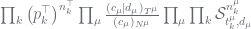
Now the theory of this configuration appears in many places but Marcus Hutter and I review it in Section 8 of an ArXiv paper, and its worked through for this case in my recent tutorial in the section “Working the n-gram Model”. The posterior distribution for the case with data at the leaf nodes is given by:

\prod_k \left(p_k^\top\right)^{n_k^\top} \prod_\mu\frac{(c_\mu|d_\mu)_{T^\mu}}{(c_\mu)_{N^\mu}} \prod_\mu\prod_k {\cal S}^{n^\mu_k}_{t^\mu_k,d_\mu}                 (2)

There are a lot of new terms here so let us review them:

(c|d)_{T} is the Pochhammer symbol (a generalised version is used, and a different notation) which is a form of rising factorial so its given by c (c+d) (c+2d) ... (c+(T-1)d); can be computed using Gamma functions
(c)_{T} a related rising factorial given by c (c+1) (c+2) ... (c+(T-1)) so it corresponds to (c_\mu|1)_{T}
\top the root node of the hierarchy
p^{\top}_k the initial/prior probability of the k-th outcome at the root
{\cal S}^{n}_{t,d} a generalised Stirling number of the second kind for discount d and counts (n,t)

Background theory for the Stirling number is reviewed in Section 5.2 of the ArXiv paper, and developed many decades ago by mathematicians and statisticians. We have C and Java libraries for this, for instance the C version is on MLOSS so its O(1) to evaluate, usually.

Now to turn this into a Gibbs sampler, we have to isolate the terms for each t^\mu_k individually. Let \theta be the parent of \mu. The constraints are:

constraint t^\mu_k \le n^\mu_k
constraint t^\mu_k>0 whenever n^\mu_k>0
propagating counts n^\theta_k = \sum_{\phi \in \theta} t^\phi_k
propagating counts t^\theta_k \le \sum_{\phi \in \theta} t^\phi_k

The propagating constraints do not apply when \mu is the root, and in this case, where $\vec{p}^\top$ is given, t_k^\top does not exist.  For \theta the parent of \mu, the constraints can be rearranged to become:

when n^\mu_k=0 t^\mu_k =0
when n^\mu_k=1 t^\mu_k =1
when n^\mu_k>1 1\le t^\mu_k \le n^\mu_k
t^\mu_k \ge t^\theta_k -\sum_{\phi \in \theta,\phi\ne \mu} t^\phi_k

The terms in Equation (2) involving t^\mu_k when \mu is not the root are:

\frac{(c_\mu|d_\mu)_{T^\mu}}{(c_\theta)_{N^\theta}} {\cal S}^{n^\mu_k}_{t^\mu_k,d_\mu}{\cal S}^{n^\theta_k}_{t^\theta_k,d_\theta} (3)

where note that t^\mu_k appears inside n^\theta_k, N^\theta and T^\mu. When \mu is the root, this becomes

\left(p_k^\top\right)^{n_k^\top} (c_\top|d_\top)_{T^\top} {\cal S}^{n^\top_k}_{t^\top_k,d_\top} (4)

The Gibbs sampler for the hierarchical model becomes as follows:

Gibbs sampler

For each node \mu do:

for each outcome k do:

sample t^\mu_k according to Equation (3) or (4) satisfying constraints in the last table above.

endfor

endfor

As noted by Teh, this can result in a very large range for t^\mu_k when n^\mu_k is large.  We overcome this by constraining t^\mu_k to be within plus or minus 10 of its last value, an approximation good enough for large n^\mu_k.

Moreover, we can initialise t^\mu_k to reasonable values by propagating up using the expected value formula from Section 5.3 of the ArXiv paper.  We only bother doing this when n^\mu_k>1.  The resultant initialisation procedure works in levels:  estimate \vec{t}^\mu at the leaves, propagate these to the \vec{n}^\mu at the next level, estimate \vec{t}^\mu at this next level, propagate these up, etc.

Initialisation

for each level, starting at the bottom do:

for each node \mu at the current level do:

for each outcome k do:

if n^\mu_k\le 1 then

t^\mu_k\leftarrow n^\mu_k

elseif  d_\mu>0 then # the PYP case

t^\mu_k\leftarrow max\left(1,floor\left(\frac{c_\mu}{d_\mu}\left(\frac{(c_\mu+d_\mu)_{n^\mu_k}}{(c_\mu)_{n^\mu_k}}-1\right)\right)\right)

else # the DP case

t^\mu_k \leftarrow max\left(1,floor\left(c_\mu\left(\psi_0 (c_\mu+n^\mu_k) - \psi_0 (c_\mu)\right)\right)\right)

\psi_0() 
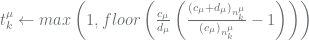
is the digamma function

endif

endfor

endfor

for each node \mu directly above current level do:

n^\mu_k = \sum_{\phi \in \mu} t^\phi_k

endfor

endfor

This represents a moderately efficient sampler for the hierarchical model.  To make this work efficiently you need to:

  • set up the data structures so the various counts, totals and parent nodes can be traversed and accessed quickly;
  • set up the sampling so leaf nodes and parents where n^\mu_k is guaranteed to be 0 or 1 can be efficiently ignored;
  • but more importantly, we also need to sample the discounts and concentrations.

Note sampling the discounts and concentrations is the most expensive part of the operation because each time you change them the counts \vec{t}^\mu also need to be resampled.  When the parameters are fixed, convergence is fast.  We will look at this final sampling task next.

h1

Training a Pitman-Yor process tree with observed data at the leaves (part 1)

November 12, 2014

A simple problem with hierarchical Pitman-Yor processes (PYPs) or Dirichlet processes (DP) is where you have a hierarchy of probability vectors and data only at the leaf nodes.  The task is to estimate the probabilities at the leaf nodes.  The hierarchy is used to allow sharing across children without resorting to Bayesian model averaging as I did for decision trees (of the Ross Quinlan variety) in my 1992 PhD thesis (journal article here) and done for n-grams with the famous Context Tree Weighting compression method.

The technique used here is somewhat similar to Katz’s back-off smoothing for n-grams but the discounts and back-off weight are estimated differently.  Yeh Whye Teh created this model originally, and it is published in an ACL 2006 paper, though the real theory is buried in an NUS technical report (yes, one of those amazing unpublished manuscripts). However, his sampler is not very good, so the purpose of this note is to explain a better algorithm.  The error in his logic is exposed in the following quote (page 16 of the amazing NUS manuscript):

However each iteration is computationally intensive as each c_{uw\cdot} and t_{uw} can potentially take on many values, and it is expensive to compute the generalized Stirling numbers s_d (c, t).

We use simple approximations and caching to overcome these problems. His technique, however, has generated a lot of interest and a lot of papers use it.  But the new sampler/estimate is a lot faster, gives substantially better predictive results, and requires no dynamic memory.  Note that when the data at the leaves is also latent, such as with clustering, topic models, or HMMs, then completely different methods are needed to enable faster mixing.  This note is only about the simplest case where the data at the leaves is observed.

The basic task is we want to estimate a probability of the k-th outcome at a node \theta, call it \hat{p}^\theta_k, by smoothing the observed data n^\theta_k at the node with the estimated probability at the parent node \phi denoted \hat{p}^\phi_k.  The formula used by Teh is as follows:

\hat{p}^\theta_k ~=~ \frac{n^\theta_k - t^\theta_k d}{N^\theta+c} + \frac{c+T^\theta \,d}{N^\theta+c} \,\, \hat{p}^\phi_k             (1)

In this, the pair (d,c) are the parameters of the PYP called discount and concentration respectively, where 0 \le d < 1 and c \ge -d.  The Ns and Ts are totals, so N^\mu=\sum_k n^\mu_k and T^\mu=\sum_k t^\mu_k for all nodes \mu in the graph.  The DP is the case where d=0.

For discount of d=0, its easy to see that for large amounts of data the probability estimate converges to the observed frequency, so this behaves well.

If the data is at the leaf nodes, where do the counts n^\mu_k for non-leaf nodes \mu come from?  Easy, they are totalled from their children’s t counts n^\mu_k=\sum_{\phi \in \mu} t^\phi_k (using \phi \in \mu to denote \phi are the children).

But what then are the t^\mu_k?  In the Chinese Restaurant Process (CRP) view of a PYP, these are the “number of tables” at the node.  To understand this, you could go and spend a few hours studying CRPs.  You don’t need to if you don’t know it already.  The way to think of it is:

The t^\mu_k are the subset of counts n^\mu_k that you will pass from the node \mu to its parent \phi in the form of a multinomial message.  So the contribution from \mu to \phi is a likelihood with the form \prod_k \phi_k^{t^\mu_k}.  The more or less counts you pass up the stronger or weaker you are making the message.

The idea is that if we expect the probability vector at \mu to be very similar to the vector at \phi, then most of the data should pass up, so t^\mu_k is close to n^\mu_k. In this case, the first term in Equation (1) shrinks and the loss is transferred via T^\mu so the parent probability contributes more to the estimate. Conversely, if the probability vector at \mu should be quite different, then only a small amount of data should pass up and t^\mu_k is closer to 1 when n^\mu_k>0.  Consequently T^\mu is smaller so the parent probability contributes less to the estimate.   Similarly, increasing the concentration makes the first term smaller and allows the parent probability to contribute more to the estimate, and vice versa.  Finally, note for the DP the t^\mu_k don’t seem to appear in Equation (1), but in reality thet do they are just hidden.  They have propagated up to the parent counts so are used in the parent probability estimate \hat{p}^\phi_k.  So the more of them there are, the more confident you are about your parent’s probability.

PYP theory and sampling has a property shared by many other species sampling distributions that this just all works.   But there is some effort in sampling the \vec{t}^\mu.

This Equation (1) is a recursive formula.  The task of estimating probabilities is now reduced to:

  1. Build the tree of nodes and populate the data in counts \vec{n}^\theta at leaf nodes \theta.
  2. Run some algorithm to estimate the \vec{t}^\mu for nodes \mu, and hence the \vec{n}^\mu for non-leaf nodes \mu.
  3. Estimate the probabilities from the root node down using Equation (1).

So the whole procedure for probability estimate is very simple, except for the two missing bits:

  • How do you estimate the \vec{t}^\mu (and thus \vec{n}^\mu for non-leaf nodes)?
  • How do you estimate the discount and concentration parameters?  By the way, we can vary these per node too!

We will look at the first of these two tasks next.

h1

Experimental results for non-parametric LDA

November 12, 2014

Swapnil Mishra and I have been testing different software for HDP-LDA, the non-parametric version of LDA first published by Teh, Jordan, Beal and Blei in JASA 2006.  Since then ever more complex and theoretical approaches have been published for this, and its a common topic in recent NIPS conferences.  We’d noticed that the LDA implementation in Mallet has an asymmetric-symmetric version which is a truncated form of HDP-LDA, and David Mimno says this has been around since 2007, though Wallach, Mimno and McCallum published their results with it in NIPS 2009.  Another fast implementation is by Sato, Kurihara, and Nakagawa in KDD 2011,  The original version some people test against is Yee Whye Teh’s implementation from 2004, Nonparametric Bayesian Mixture Models – release 2.1.  This is impressive because it does “slow” Gibbs sampling and still works OK!

We’ve had real trouble comparing different published work because everyone has different ways of measuring perplexity, their test sets are hard to reconstruct, and sometimes their code works really badly and we’ve been unable to get realistic looking results.

Our KDD paper did some comparisons.  We’re re-running things more carefully now.  To compare against Sato et al.‘s results he kindly sent us his original data sets.   Their experimental work was thorough, and precisely written up so its a good one to compare with.  We’ve then re-run Mallet with their ASYM-SYM option to compare and our own two versions of HDP-LDA and our fully non-parametric version NP-LDA (puts a Pitman-Yor process on the word distributions and a Dirichlet process on the topic distributions).  Results in the plot below, lower perplexity is better.  Not sure about Teh’s original 2004 code but our experience from other runs would be it doesn’t match these others.

pcvb0Most of these are with 300 topics.  We’re impressed with how well the others performed.  Mallet is a lot faster because they use some very clever sampling designed for LDA.  Ours is the next fastest because our samplers are much better and it runs moderately well in 8 cores (cheating really).  More details on the comparison in a forth-coming paper.

h1

Lancelot James on the history of the Pitman-Yor Process

November 10, 2014

Those of us in Machine Learning (read Computer Science) departments rely on the work of many statisticians.  While Jim Pitman (UCB) and colleagues has been instrumental in developing the fundamental theory, other statisticians such as Lancelot James (HKUST) have been extending the work and interpreting it so the rest of us can understand it.  Marcus Hutter (ANU) developed a bunch of formula, and I remember him being shattered to discover his toughest “exact formula for the second order Stirling number” was published by Toscano in 1939, and Lancelot cites Halmos 1944 on stick-breaking!

So its important to know our history.  Here is Lancelot’s short history of the Pitman-Yor Process, he wrote during correspondence with us, and my students and I are most grateful for his many insights (some edits by me):

  • The process arises from a comprehensive study of excursion lengths on Markov processes, where an excursion length is the time from one zero-crossing to the next:
    •  Excursions can either be positive or negative. So the (P k) represent the length of excursions of a process on [0,1].  The sign of the excursion is not reflected in the law of (P k). In fact it is independent of the length.
    • A class of Bessel Processes indexed by a parameter 0 ≤ α < 1 in a series of works of Jim Pitman and Marc Yor and co-authors during the 1980’s and 1990’s, generalizing results for Brownian motion (which is the α = 1/2 case).
    • The study of (P k) following a two parameter Poisson-Dirichlet distribution with parameters (α, θ) denoted as PD(α, θ). PD(1/2, 0), corresponds to Brownian Motion and PD(1/2, 1/2), corresponds to Brownian Bridge.
  • Its stick-breaking representation is formally derived in Perman, Pitman and Yor (1992):
  • This process, but not Bayesian aspects of it, is later discussed by Pitman and Yor:
  • The corresponding random distribution function is treated in a formal Bayesian setting by Pitman:
  • See also:
    • Pitman, J. Combinatorial stochastic processes. Lecture Notes in Mathematics Vol. 1875, x+256, Springer-Verlag, Berlin (2006). Lectures from the 32nd Summer School on Probability Theory held in Saint-Flour, July 7–24, 2002, With a foreword by Jean Picard.
    • Pitman, Jim (2003) “Poisson-Kingman partitions” in Science and Statistics: A Festschrift for Terry Speed, D. R. Goldstein editor, Lecture Notes – Monograph Series Vol. 30, 1-34, Institute of Mathematical Statistics, Beachwood, OH (2003).
  • Ishwaran and James showed how such processes could be used practically in complex Bayesian mixture models and also were the ones who first called these processes Pitman-Yor processes:
    • Ishwaran, Hemant, and Lancelot F. James, ”Gibbs sampling methods for stick-breaking priors,” Journal of the American Statistical Association 96.453 (2001).
    • Ishwaran, Hemant, and Lancelot F. James, “Generalized weighted Chinese restaurant processes for species sampling mixture models,” Statistica Sinica 13.4 (2003): 1211-1236.
  • Arguably, it is their 2001 paper that helped to popularize the wide usage of stick-breaking representations and also of course the Pitman-Yor process itself within the BNP and the ML communities. Goldwater, Griffiths and Johnson were the first to point out that the Pitman-Yor process proved to be superior to the Dirichlet Process for language applications involving certain types of power law behavior.
    • Goldwater, Sharon, Tom Griffiths, and Mark Johnson. ”Interpolating between types and tokens by estimating power-law generators.” Advances in Neural Information Processing Systems 18 (2006): 459.
      This makes the PY process an important model in ML/NLP applications.
  • Arratia, Barbour and Tavar ́e in contrast one would note the DP is a much better process to use if one were trying to model logarithmic behavior as illustrated in
    • Arratia, R., A. D. Barbour, and S. Tavar ́e, Logarithmic Combinatorial Structures: A Probabilistic Approach, 2003, EMS Monographs in Mathematics 1.
  • So this points out that not all processes are appropriate in all cases.
h1

Information for candidate research students

November 2, 2014

I wrote a page for candidate research students here.  Always happy to hear from you folks.