Dirichlet-multinomial distribution versus Pitman-Yor-multinomial

March 18, 2015

If you’re familiar with the Dirichlet distribution as the workhorse for discrete Bayesian modelling, then you should know about the Dirichlet-multinomial. This is what happens when you combine a Dirichlet with a multinomial and integrate/marginalise out the common probability vector.

Graphically, you have a probability vector $\vec\theta$ that is the mean for a probability vector $\vec{p}$ . You then have data, a count vector $\vec{n}$ , drawn using a multinomial distribution with mean $\vec{p}$ . If we integrate out the vector $\vec{p}$ then we get the Dirichlet-multinomial.

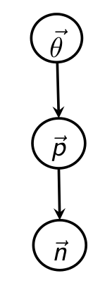
The standard formulation is to have:
$\vec{p} \sim \mbox{Dirichlet}\left(\alpha,\vec\theta\right) ~~~~~~~~~~~~ \vec{n} \sim \mbox{Multinomial}\left(\vec{p},N\right)$

Manipulating this, we get the distribution for the Dirichlet-multinomial:
$p\left( \vec{n}\,\middle\vert\, \alpha,\vec\theta,N, \mbox{\small Dirichlet-multi.}\right)$
$~~~~~~~~~~~~=~ \frac{1}{\mbox{\small Beta}(\alpha \vec\theta)}{N \choose \vec{n} } \int_{\mbox{\scriptsize simplex}} \prod_k p_{k}^{n_k+\alpha \theta_k-1} \mbox{d}\vec{p}$
$~~~~~~~~~~~~=~ {N \choose \vec{n} } \frac{\mbox{\small Beta}(\vec{n}+\alpha \vec\theta)}{\mbox{\small Beta}(\alpha \vec\theta)}$

Now we will rewrite this into the Pochhammer symbol notation we use for Pitman-Yor marginals,

$(c\|d)_{T}$	is the Pochhammer symbol (a generalised version is used, and a different notation) which is a form of rising factorial so its given by $c (c+d) (c+2d) ... (c+(T-1)d)$ ; can be computed using Gamma functions
$(c)_{T}$	(special case) a related rising factorial given by $c (c+1) (c+2) ... (c+(T-1))$ so it corresponds to $(c\|1)_{T}$

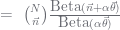
The Beta functions simplify to yield the Dirichlet-multinomial in Pochhammer symbol notation:

$p\left( \vec{n}\,\middle\vert\, \alpha,\vec\theta,N,\mbox{\small Dirichlet-multi.}\right) ~=~ {N \choose \vec{n} } \frac{1}{(\alpha)_N} \prod_{k=1}^K (\alpha\theta_k)_{n_k}$

Now lets do the same with the Pitman-Yor process (PYP).
$\vec{p} \sim \mbox{PYP}\left(d,\alpha,\vec\theta\right) ~~~~~~~~~~~~ \vec{n} \sim \mbox{Multinomial}\left(\vec{p},N\right)$

The derivation of the combination is more detailed but is found in the Buntine Hutter Arxiv report or my tutorials. For this, you have to introduce a new latent vector $\vec{t}$ where $t_k$ represents the subset of the count $n_k$ that will be passed up from the $\vec{p}$ -node up to the $\vec{\theta}$ -node to convey information about the data $\vec{n}$ . Keep this phrase in mind. It will be explained a bit later. These $\vec{t}$ are constrained as follows:

constraint	$t_k \le n_k$
constraint	$t_k>0$ whenever $n_k>0$
total	$N=\sum_k n_k$
total	$T=\sum_k t_k$

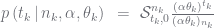
With these, we get the PYP-multinomial in Pochhammer symbol notation:

$p\left( \vec{n},\vec{t}\,\middle\vert\, d,\alpha,\vec\theta,N,\mbox{\small PYP-multi.}\right) ~=~ {N \choose \vec{n}} \frac{(\alpha|d)_T}{(\alpha)_N} \prod_{k = 1}^K \mathcal{S}_{t_k, d}^{n_k} \theta_k^{t_k}$

You can see the three main differences. With the PYP:

the terms in $\vec\theta$ appear as simple powers, just like a multinomial likelihood, so this form is readily used in a hierarchy;
you now have to work with the generalised Stirling numbers $\mathcal{S}_{t_k, d}^{n_k}$ ; and
you have to introduce the new latent vector $\vec{t}$ .

The key thing is that $\vec\theta$ only appears in the expression $\prod_{k=1}^K \theta_k^{t_k}$ which is a multinomial likelihood. So, as said earlier, $t_k$ represents the subset of the count $n_k$ that will be passed up from the $\vec{p}$ -node up to the $\vec{\theta}$ -node. If $\vec{t}=\vec{n}$ then all the data is passed up, and the likelihood looks like $\prod_{k=1}^K \theta_k^{n_k}$ , which is what you would get if $\vec{p}=\vec{\theta}$ .

If we use a Dirichlet process (DP) rather than a PYP, the only simplification is that $(\alpha|d)_T$ simplifies to $\alpha^T$ . This small change means that the above formula can be rewritten as:

$p\left( \vec{n},\vec{t}\,\middle\vert\, \alpha,\vec\theta,N,\mbox{\small DP-multi.}\right) ~=~ {N \choose \vec{n}} \frac{1}{(\alpha)_N} \prod_{k = 1}^K \mathcal{S}_{t_k, d}^{n_k}(\alpha\theta_k)^{t_k}$

This has quite broad implications as the $t_k$ are now independent variables! In fact, their posterior distribution takes the form:

$p\left( t_k\,\middle\vert\, n_k,\alpha,\theta_k\right)~=~ \mathcal{S}_{t_k, 0}^{n_k} \frac{(\alpha\theta_k)^{t_k}}{ (\alpha\theta_k)_{n_k} }$

The penalty for using the PYP or DP is that you now have to work with the generalised Stirling numbers and the latent vector $\vec{t}$ . With the right software, the Stirling numbers are easy to handle. While my students have built their own Java packages for that, I use a C library available from MLOSS. The latent vectors $\vec{t}$ at each node require different sampling algorithms.

Now one final note, this isn’t how we implement these. Sampling the full range of $\vec{t}$ is too slow … there are too many possibilities. Moreover, if sampling $\vec{t}$ , you ignore the remainder of the hierarchy. For fast mixing of Markov chains, you want to sample a cluster of related variables. The hierarchical CRP does this implicitly as it resamples and samples up and down the parent hierarchy. So to achieve this same effect using the marginalised posteriors above we have too Booleanise (turn into a Boolean) the $\vec{t}$ ‘s and sample a cluster of related Booleans up and down the hierarchy. We figure out how to do this in 2011, paper at ECML.

Posted in theory | Tagged PYP |

Bayesian Models