Training a Pitman-Yor process tree with observed data at the leaves (part 2)

November 13, 2014

So here is a recap of the previous post:

A simple problem with hierarchical Pitman-Yor processes (PYPs) or Dirichlet processes (DP) is where you have a hierarchy of probability vectors and data only at the leaf nodes. The task is to estimate the probabilities at the leaf nodes. The hierarchy is used to allow sharing across children …

We have a tree of nodes which have probability vectors. The formula used estimates a probability for node $\theta$ from its parent $\phi$ as follows:

$\hat{p}^\theta_k ~=~ \frac{n^\theta_k - t^\theta_k d}{N^\theta+c} + \frac{c+T^\theta \,d}{N^\theta+c} \,\, \hat{p}^\phi_k$ (1)

In this, the pair $(d,c)$ are the parameters of the PYP called discount and concentration respectively, where $0 \le d < 1$ and $c \ge -d$ . The $t^\mu_k$ are magical auxiliary (latent) counts that make the PYP samplers work efficiently. They are, importantly, constrained by their corresponding counts, and the counts are computed up from the leaves up (using $\phi \in \mu$ to denote $\phi$ are the children of $\mu$ ). The $N$ s and $T$ s are totals. These relationships are summarised in the table below.

constraint	$t^\mu_k \le n^\mu_k$
constraint	$t^\mu_k>0$ whenever $n^\mu_k>0$
propagating counts	$n^\mu_k=\sum_{\phi \in \mu} t^\phi_k$
total	$N^\mu=\sum_k n^\mu_k$
total	$T^\mu=\sum_k t^\mu_k$

It is important to note here how the counts propagate upwards. In some smoothing algorithms, propagation is $n^\mu_k=\sum_{\phi \in \mu} n^\phi_k$ . This is not the case with us. Here the non-leaf nodes represent priors on the leaf nodes, they do not represent alternative models. PYP theory tells us how to make inference about these priors.

Now the theory of this configuration appears in many places but Marcus Hutter and I review it in Section 8 of an ArXiv paper, and its worked through for this case in my recent tutorial in the section “Working the n-gram Model”. The posterior distribution for the case with data at the leaf nodes is given by:

$\prod_k \left(p_k^\top\right)^{n_k^\top} \prod_\mu\frac{(c_\mu|d_\mu)_{T^\mu}}{(c_\mu)_{N^\mu}} \prod_\mu\prod_k {\cal S}^{n^\mu_k}_{t^\mu_k,d_\mu}$ (2)

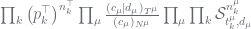
There are a lot of new terms here so let us review them:

$(c\|d)_{T}$	is the Pochhammer symbol (a generalised version is used, and a different notation) which is a form of rising factorial so its given by $c (c+d) (c+2d) ... (c+(T-1)d)$ ; can be computed using Gamma functions
$(c)_{T}$	a related rising factorial given by $c (c+1) (c+2) ... (c+(T-1))$ so it corresponds to $(c_\mu\|1)_{T}$
$\top$	the root node of the hierarchy
$p^{\top}_k$	the initial/prior probability of the k-th outcome at the root
${\cal S}^{n}_{t,d}$	a generalised Stirling number of the second kind for discount $d$ and counts $(n,t)$

Background theory for the Stirling number is reviewed in Section 5.2 of the ArXiv paper, and developed many decades ago by mathematicians and statisticians. We have C and Java libraries for this, for instance the C version is on MLOSS so its O(1) to evaluate, usually.

Now to turn this into a Gibbs sampler, we have to isolate the terms for each $t^\mu_k$ individually. Let $\theta$ be the parent of $\mu$ . The constraints are:

constraint	$t^\mu_k \le n^\mu_k$
constraint	$t^\mu_k>0$ whenever $n^\mu_k>0$
propagating counts	$n^\theta_k = \sum_{\phi \in \theta} t^\phi_k$
propagating counts	$t^\theta_k \le \sum_{\phi \in \theta} t^\phi_k$

The propagating constraints do not apply when $\mu$ is the root, and in this case, where $\vec{p}^\top$ is given, $t_k^\top$ does not exist. For $\theta$ the parent of $\mu$ , the constraints can be rearranged to become:

when $n^\mu_k=0$	$t^\mu_k =0$
when $n^\mu_k=1$	$t^\mu_k =1$
when $n^\mu_k>1$	$1\le t^\mu_k \le n^\mu_k$ $t^\mu_k \ge t^\theta_k -\sum_{\phi \in \theta,\phi\ne \mu} t^\phi_k$

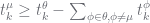
The terms in Equation (2) involving $t^\mu_k$ when $\mu$ is not the root are:

$\frac{(c_\mu|d_\mu)_{T^\mu}}{(c_\theta)_{N^\theta}} {\cal S}^{n^\mu_k}_{t^\mu_k,d_\mu}{\cal S}^{n^\theta_k}_{t^\theta_k,d_\theta}$ (3)

where note that $t^\mu_k$ appears inside $n^\theta_k$ , $N^\theta$ and $T^\mu$ . When $\mu$ is the root, this becomes

$\left(p_k^\top\right)^{n_k^\top} (c_\top|d_\top)_{T^\top} {\cal S}^{n^\top_k}_{t^\top_k,d_\top}$ (4)

The Gibbs sampler for the hierarchical model becomes as follows:

Gibbs sampler

For each node $\mu$ do:

for each outcome $k$ do:

sample $t^\mu_k$ according to Equation (3) or (4) satisfying constraints in the last table above.

endfor

endfor

As noted by Teh, this can result in a very large range for $t^\mu_k$ when $n^\mu_k$ is large. We overcome this by constraining $t^\mu_k$ to be within plus or minus 10 of its last value, an approximation good enough for large $n^\mu_k$ .

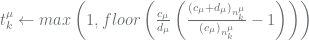
Moreover, we can initialise $t^\mu_k$ to reasonable values by propagating up using the expected value formula from Section 5.3 of the ArXiv paper. We only bother doing this when $n^\mu_k>1$ . The resultant initialisation procedure works in levels: estimate $\vec{t}^\mu$ at the leaves, propagate these to the $\vec{n}^\mu$ at the next level, estimate $\vec{t}^\mu$ at this next level, propagate these up, etc.

Initialisation

for each level, starting at the bottom do:

for each node $\mu$ at the current level do:

for each outcome $k$ do:

if $n^\mu_k\le 1$ then

$t^\mu_k\leftarrow n^\mu_k$

elseif $d_\mu>0$ then # the PYP case

$t^\mu_k\leftarrow max\left(1,floor\left(\frac{c_\mu}{d_\mu}\left(\frac{(c_\mu+d_\mu)_{n^\mu_k}}{(c_\mu)_{n^\mu_k}}-1\right)\right)\right)$

else # the DP case

$t^\mu_k \leftarrow max\left(1,floor\left(c_\mu\left(\psi_0 (c_\mu+n^\mu_k) - \psi_0 (c_\mu)\right)\right)\right)$

# $\psi_0()$ is the digamma function

endif

endfor

endfor

for each node $\mu$ directly above current level do:

$n^\mu_k = \sum_{\phi \in \mu} t^\phi_k$

endfor

endfor

This represents a moderately efficient sampler for the hierarchical model. To make this work efficiently you need to:

set up the data structures so the various counts, totals and parent nodes can be traversed and accessed quickly;
set up the sampling so leaf nodes and parents where $n^\mu_k$ is guaranteed to be 0 or 1 can be efficiently ignored;
but more importantly, we also need to sample the discounts and concentrations.

Note sampling the discounts and concentrations is the most expensive part of the operation because each time you change them the counts $\vec{t}^\mu$ also need to be resampled. When the parameters are fixed, convergence is fast. We will look at this final sampling task next.

Posted in theory |

One comment

[…] We will look at the first of these two tasks next. […]
by Training a Pitman-Yor process tree with observed data at the leaves (part 1) | Topical Issues November 13, 2014 at 8:35 am

Reply

Bayesian Models